Markov Information Binary Sequences Based on Piecewise Linear Chaotic Maps
Get 1000000 0FP0EXP Token to remove widget entirely!
Get 500000 0FP0EXP Token to remove my NFTS advertisements!
0. Note
This is the third assignment from my Masters Applied Digital Information Theory Course which has never been published anywhere and I, as the author and copyright holder, license this assignment customized CC-BY-SA where anyone can share, copy, republish, and sell on condition to state my name as the author and notify that the original and open version available here.
1. Introduction
On the first assignment we produced a chaotic sequence based skew tent map by showing that output sequence is uncontrollable as on the chaos theory. A large sequence produced by skew tent map is uniformly distributed. On the second assignment we produce a memoryless binary sequence based on the first assignment’s skew tent map based chaotic sequence. The probability of 0, 1, 00, 01, 10, 11, and the Markov chain is analyze. Finally the entropy is calculated based on the critical points of each data and find the correlation between the entropy and expected compression ratio. This time the same method on assignment 2 is used but change the assignment 1 of not using skew tent map but piecewise linear map.
2. Piecewise Linear Chaotic Map
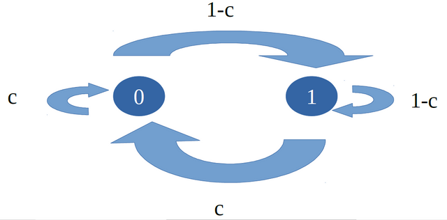
Figure 1. Markov’s Chain
The design procedure of Markov Source we choose 4 values p1, and p2 based on Figure 1. Then can obtain the value c (steady state probability) with the formula c=P(0)=P2/(P1+P2), and then we can find the slope a=1/(1-(p1+p2)). The limitation here is we cannot choose the value that satisfy p1+p2 = 1. We are now ready to design the chaotic map. Basic knowledge on line equation is necessary here the one that refers to the equation y = ax + d where a is the slope that we calculated. There will be 3 lines and at least a positive and negative must be use. Each line we calculate its slope. For Figure 2 we calculate slope a = (y2 – y1)/(x2 – x1). For a=(c-0)/(c-c1)from point x,y of (c1,0) and (c,c). From the equation we can define c1=c-c/a. There’s also another slope for a=(1-c)/(c2-c)from point (c,c) and (c2,1) which then we can define c2=c+(1-c)/a. With the first line as negative slope the length proportion of c1:d1 = 1:1-c thus d1 = c1(1-c), and for the third line also negative slope 1-c2:1-d2 = 1:c which we can define d2 = 1+(1-c)c. That’s almost all the equation we need, next is to find slope a1 and a2.
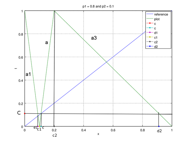
Figure 2a. Plot of p1 = 0.8 , p2 = 0.1
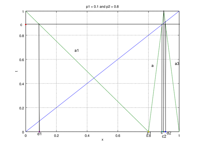
Figure 2b. Plot of p1 = 0.1, p2 = 0.8
For both figure the method to find a1 and a3 is the same which is by using 2 points (x1,y1) and (x2,y2) with calculation slope = (y2 – y1)/(x2 – x1). We use point (d1,c) and (c1,0) for a1. a1=(0-c)/(c1-d1), as for a3 we use (c2,1) and (d2,c) a3=(c-1)/(d2-c2). Finally we can form each line y1, y2, and y3, using equation y – y1 = a(x – x1), but for the map y is regarded as t (it’ll be t = a(x-x1) + y1). We then use the following equation to generate the chaotic sequence of p1+p2 < 1.
t = (a1(x-d1))+c for (0⩽x < c1)
t = a(x-c1) for (c1⩽x < c2)
t= a3(x-c2)+1 for (c2⩽x < 1)
For p1+p2 < 1 on the other hand have to change some equation to do the slope a is negative.
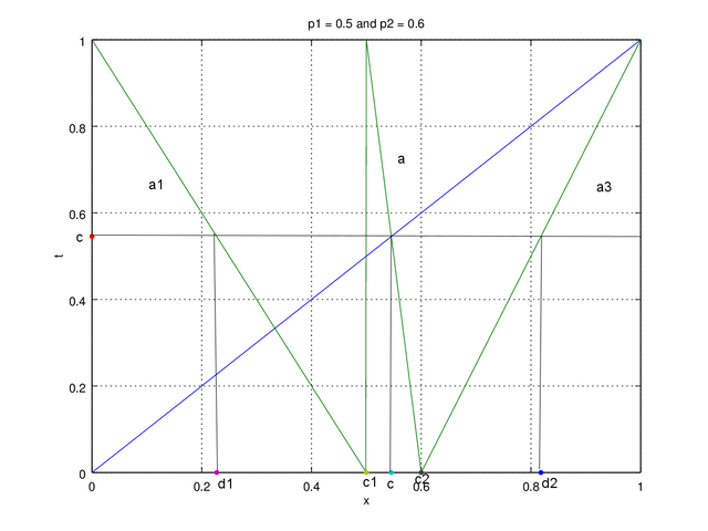
Figure 3a. Plot of p1 = 0.5 , p2 = 0.6
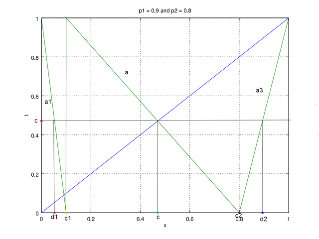
Figure 3b. Plot of p1 = 0.9, p2 = 0.8
On Figure 3 we change one slope for it to be positive, and here we chose a3. Since the slope a2 changes to negative the equation c1 and c2 changes as well, a = (y2 – y1)/(x2 – x1) a=(c-1)/(c-c1)from point x,y of (c1,1) and (c,c). From the equation we can define c1=c-(c-1)/a. C2 changes as well a=(0-c)/(c2-c) from point (c2,0) and (c,c) which then we can define c2=c-c/a. The slope on a1 is still negative, so no changes for d1, but third line we change to positive slope 1-c2:1-d2 = 1:1-c which we can define d2 = 1-(1-c2)(1-c). The last change is on a3=(c-0)/(d2-dc) using point (c2,0) and (d2,c). Not to forget a changes slop recently so t had to be modified based on t = a(x-x1)+y1, the equation then becomes:
t = (a1(x-d1))+c for (0⩽x < c1)
t = a(x-c1)+1 for (c1⩽x < c2)
t = a3(x-c2) for (c2⩽x < 1)
Now we can generate the chaotic sequence on Figure 4. We can see that for p1+p2 < 1 seems more periodic. Lastly on this section we would like to show that the distribution is uniform on Figure 5.
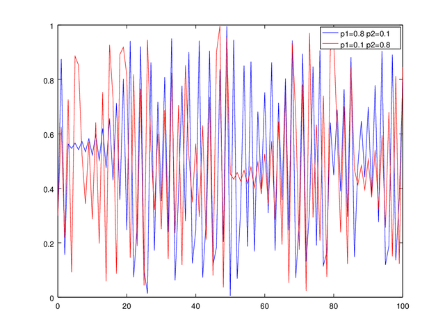
Figure 4a. Generated chaotic sequence of p1 = 0.8 p2 = 0.1 and p1 = 0.1 p2 = 0.8
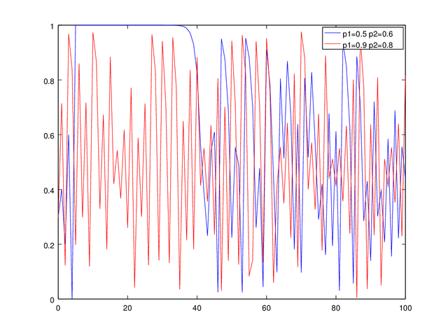
Figure 4b. Generated chaotic sequence of p1 = 0.5 p2 = 0.6 and p1 = 0.9 p2 = 0.8
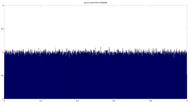
Figure 5a. Uniform distribution of p1 = 0.1 p2 = 0.8 N = 1000000
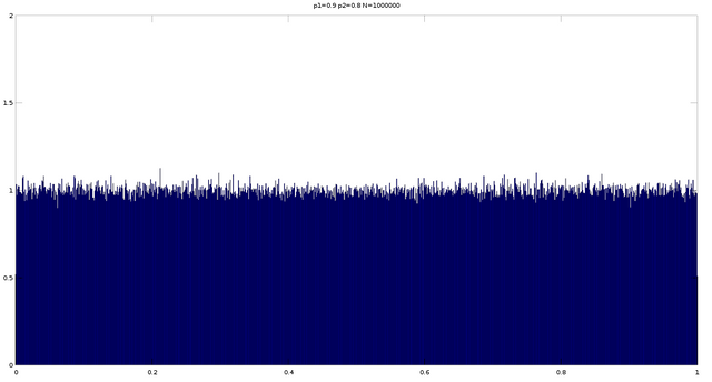
Figure 5b. Uniform distribution of p1 =0.9 p2 = 0.8 N = 1000000
3. Binary Sequences
| After that we do the same as assignment 2, generating the binary sequences and counting the 0s and 1s. The result below are as the theory where P(0)=c, P(1)=1-c, P(0 | 0)=1-p1, P(0 | 1)=p1, P(1 | 0)=p2, P(1 | 1)=1-p2, P(00)=P(0 | 0)*P(0), P(01)=P(0 | 1)*P(1), P(10)=P(1 | 0)*P(1), P(11)=P(1 | 1)*P(1). |
| P1 = 0.1p2 = 0.8 | Theory | Practice | P1 = 0.8p2 = 0.1 | Theory | Practice |
|---|---|---|---|---|---|
| 0s | - | 888925 | 0s | - | 110631 |
| 1s | - | 111076 | 1s | - | 889370 |
| 00s | - | 800154 | 00s | - | 21997 |
| 01s | - | 88770 | 01s | - | 88634 |
| 10s | - | 88770 | 10s | - | 88634 |
| 11s | - | 22306 | 11s | - | 800735 |
| P(0) | 0.888889 | 0.888924 | P(0) | 0.111111 | 0.110631 |
| P(1) | 0.111111 | 0.111076 | P(1) | 0.888889 | 0.889369 |
| P(00) | 0.800000 | 0.800153 | P(00) | 0.022222 | 0.021997 |
| P(01) | 0.088889 | 0.088770 | P(01) | 0.088889 | 0.088634 |
| P(10) | 0.088889 | 0.088770 | P(10) | 0.088889 | 0.088634 |
| P(11) | 0.022222 | 0.022306 | P(11) | 0.800000 | 0.800734 |
| P(0|0) | 0.900000 | 0.900137 | P(0|0) | 0.200000 | 0.198832 |
| P(0|1) | 0.800000 | 0.799183 | P(0|1) | 0.100000 | 0.099659 |
| P(1|0) | 0.100000 | 0.099862 | P(1|0) | 0.800000 | 0.801168 |
| P(1|1) | 0.200000 | 0.200817 | P(1|1) | 0.900000 | 0.900340 |
| Entrophy | 0.497099 | 0.496884 | Entrophy | 0.497099 | 0.495759 |
| Filesize (Byte) | 1,000,000 | Filesize (Byte) | 1,000,000 | ||
| Compressed File | 100296 | Compressed File | 100037 | ||
| Compression Rate | 0.1 | Compression Rate | 0.1 | ||
| P1 = 0.5p2 = 0.6 | Theory | Practice | P1 = 0.9p2 = 0.8 | Theory | Practice |
| 0s | - | 544416 | 0s | - | 529516 |
| 1s | - | 455585 | 1s | - | 470485 |
| 00s | - | 271392 | 00s | - | 106222 |
| 01s | - | 273024 | 01s | - | 423294 |
| 10s | - | 273024 | 10s | - | 423293 |
| 11s | - | 182561 | 11s | - | 47191 |
| P(0) | 0.545455 | 0.544415 | P(0) | 0.529412 | 0.529515 |
| P(1) | 0.454545 | 0.455585 | P(1) | 0.470588 | 0.470485 |
| P(00) | 0.272727 | 0.271392 | P(00) | 0.105882 | 0.106222 |
| P(01) | 0.272727 | 0.273024 | P(01) | 0.423529 | 0.423294 |
| P(10) | 0.272727 | 0.273023 | P(10) | 0.423529 | 0.423293 |
| P(11) | 0.181818 | 0.182561 | P(11) | 0.047059 | 0.047191 |
| P(0|0) | 0.500000 | 0.498501 | P(0|0) | 0.200000 | 0.200602 |
| P(0|1) | 0.600000 | 0.599282 | P(0|1) | 0.900000 | 0.899697 |
| P(1|0) | 0.500000 | 0.501497 | P(1|0) | 0.800000 | 0.799396 |
| P(1|1) | 0.400000 | 0.400718 | P(1|1) | 0.100000 | 0.100303 |
| Entropy | 0.986796 | 0.986953 | Entropy | 0.602901 | 0.604017 |
| Filesize (Byte) | 1,000,000 | Filesize (Byte) | 1,000,000 | ||
| Compressed File | 159550 | Compressed File | 110189 | ||
| Compression Rate | 0.16 | Compression Rate | 0.11 | ||
We also perform entropy calculation of the generated binary sequence. We chose to compress the file into format “.tar.gz” one of famous compression in Linux, but this time we use the reversed formula of the second assignment for the compression rate CompressionRate=CompressedFile/OriginalFile thus got the reversed graph, although the meaning is still the same. The lower the compression rate the greater the compressed file, thus higher entropy limits the how far a file can be compressed as on Figure 6.
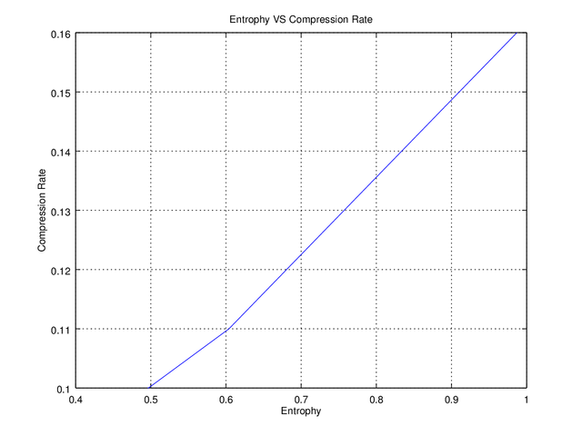
Figure 6. Entropy Vs Compression Ratio
4. Conclusion
Just as the second assignment the probability of 0s and 1s generated matched the theory. We use reversed equation for compression rate and the as expected the graph become backward thought it is the same thing that lower entropy allows greater compression. The difference in this assignment is that we used piecewise linear chaotic binary sequence which is more complex than skew tent map but allows various map design. This opens possibility to produce different kinds of sequences.
5. Source Code
The source code again is written in Octave and Matlab type language. The script this time is manual so better edit the script and change the values of you want to use it. Next time I might consider uploading the program to available online.
close all
clear
clc

x = 0:.001:1;

p1 = 0.9; p2 = 0.8;
c = p2/(p1+p2);
a = 1/(1-(p1+p2));

if p1+p2 < 1 %positive slope
 c1 = c-(c/a);
 c2 = c+((1-c)/a );
 d1 = c1*(1-c); %(we chose negative slope)
 d2 = 1-((1-c2)*c); %(we chose negative slope)

 a1 = -c/(c1-d1); %slope a = y2 - y1 / x2 - x1 (we chose negative)
 a2 = a; %positive slope
 a3 = (c-1)/(d2-c2); % (we chose negative slope)

 i = 0;

 for i = 1:length(x)
  if x(i) >= 0 && x(i) < c1
   t(i) = (a1*(x(i)-d1))+c;
  elseif x(i) >= c1 && x(i) < c2
   t(i)  = a2*(x(i)-c1);
  else
   t(i) = (a3*(x(i)-c2))+1;
  end
 end
 figure
 plot(x,x,x,t,0,c,c,0,d1,0,c1,0,c2,0,d2,0);
 grid on;
 %title('p1 = 0.1 and p2 = 0.8');
 xlabel('x');
 ylabel('t');
 %legend('reference', 'plot', 'c', 'c', 'd1', 'c1', 'c2', 'd2');
 ylim([0 1]);

 N = 1000000;
 X(1) = 0.3;

 for i = 1:N
  if X(i) >= 0 && X(i) < c1
   X(i+1) = (a1*(X(i)-d1))+c;
  elseif X(i) >= c1 && X(i) < c2
   X(i+1)  = a2*(X(i)-c1);
  else
   X(i+1) = (a3*(X(i)-c2))+1;
  end
 end

 figure
 plot(0:length(X)-1,X);

 figure
 hist(X,x,length(x));
 %title('p1=0.1 p2=0.8 N=1000000');
 xlim([0 1]);
 ylim([0 2]);

 P0_theory = c;
 P1_theory = 1-c;
 P1l0_theory = p1;
 P0l1_theory = p2;
 P0l0_theory = 1-p1;
 P1l1_theory = 1-p2;
 P01_theory = P0l1_theory*P1_theory;
 P10_theory = P1l0_theory*P0_theory;
 P00_theory = P0l0_theory*P0_theory;
 P11_theory = P1l1_theory*P1_theory;
 H_theory = ((p2/(p1+p2))*((-p1*log2(p1))-((1-p1)*log2(1-p1)))) + ((p1/(p1+p2))*((-p2*log2(p2))-((1-p2)*log2(1-p2))));

 fprintf('P(0) in theory is %f\n', P0_theory);
 fprintf('P(1) in theory is %f\n', P1_theory);
 fprintf('P(00) in theory is %f\n', P00_theory);
 fprintf('P(01) in theory is %f\n', P01_theory);
 fprintf('P(10) in theory is %f\n', P10_theory);
 fprintf('P(11) in theory is %f\n', P11_theory);
 fprintf('P(0|0) in theory is %f\n', P0l0_theory);
 fprintf('P(0|1) in theory is %f\n', P0l1_theory);
 fprintf('P(1|0) in theory is %f\n', P1l0_theory);
 fprintf('P(1|1) in theory is %f\n', P1l1_theory);
 fprintf('Entropy in theory is %f\n\n', H_theory);
 t = c;
 binary = X >= t;
 save("binary_sequence.dat", "binary");

 P0_practical = P1_practical = P00_practical = P01_practical = P10_practical = P11_practical = 0;

 for i = 1:length(binary)
  if binary(i) == 0
   P0_practical += 1;
  else
   P1_practical += 1;
  end

  if i == length(binary)
   break;
  end

  if binary(i) == 0 && binary(i+1) == 0
   P00_practical += 1;
  elseif binary(i) == 0 && binary(i+1) == 1
   P01_practical += 1;
  elseif binary(i) == 1 && binary(i+1) == 0
   P10_practical += 1;
  else
   P11_practical += 1;
  end
 end

 P0l0_practical = ((P00_practical/length(binary))/(P0_practical/length(binary)));
 P0l1_practical = ((P01_practical/length(binary))/(P1_practical/length(binary)));
 P1l0_practical = ((P10_practical/length(binary))/(P0_practical/length(binary)));
 P1l1_practical = ((P11_practical/length(binary))/(P1_practical/length(binary)));
 H_pratical = ((P0l1_practical/(P1l0_practical+P0l1_practical))*((-P1l0_practical*log2(P1l0_practical))-((P0l0_practical)*log2(P0l0_practical)))) + ((P1l0_practical/(P1l0_practical+P0l1_practical))*((-P0l1_practical*log2(P0l1_practical))-((P1l1_practical)*log2(P1l1_practical))));

 fprintf('The number of 0s = %d, P(0) in practice is %f\n', P0_practical, P0_practical/length(binary));
 fprintf('The number of 1s = %d, P(1) in practice is %f\n', P1_practical, P1_practical/length(binary));
 fprintf('The number of 00s = %d, P(00) in practice is %f\n', P00_practical, P00_practical/length(binary));
 fprintf('The number of 01s = %d, P(01) in practice is %f\n', P01_practical, P01_practical/length(binary));
 fprintf('The number of 10s = %d, P(10) in practice is %f\n', P10_practical, P10_practical/length(binary));
 fprintf('The number of 11s = %d, P(11) in practice is %f\n', P11_practical, P11_practical/length(binary));
 fprintf('P(0|0) in practice is %f\n', P0l0_practical);
 fprintf('P(0|1) in practice is %f\n', P0l1_practical);
 fprintf('P(1|0) in practice is %f\n', P1l0_practical);
 fprintf('P(1|1) in practice is %f\n', P1l1_practical);
 fprintf('Entropy in practice is %f\n\n', H_pratical);

elseif p1+p2 > 1 % negative lope
 c1 = c-((c-1)/a);
 c2 = c-(c/a);

 d1 = c1*(1-c); % we chose negative slope
 d2 = 1-((1-c2)*(1-c)); % we chose positive slope

 a1 = -c/(c1-d1); %slope a = y2 - y1 / x2 - x1 (we chose negative)
 a2 = a; % negative lope
 a3 = c/(d2-c2); %(we chose negative)

 for i = 1:length(x)
  if x(i) >= 0 && x(i) < c1
   t(i) = (a1*(x(i)-d1))+c;
  elseif x(i) >= c1 && x(i) < c2
   t(i)  =(a2*(x(i)-c1))+1;
  else
   t(i) = a3*(x(i)-c2);
  end
 end
 figure
 plot(x,x,x,t,0,c,c,0,d1,0,c1,0,c2,0,d2,0);
 grid on;
 %title('p1 = 0.9 and p2 = 0.8');
 xlabel('x');
 ylabel('t');
 %legend('reference', 'plot', 'c', 'c', 'd1', 'c1', 'c2', 'd2');
 ylim([0 1]);

 N = 1000000;
 X(1) = 0.3;

 for i = 1:N
  if X(i) >= 0 && X(i) < c1
   X(i+1) = (a1*(X(i)-d1))+c;
  elseif X(i) >= c1 && X(i) < c2
    X(i+1)  =(a2*(X(i)-c1))+1;
  else
     X(i+1) = a3*(X(i)-c2);
  end
 end

 figure
 plot(0:length(X)-1,X);

 figure
 hist(X,x,length(x));
 %title('p1=0.9 p2=0.8 N=1000000');
 xlim([0 1]);
 ylim([0 2]);

 P0_theory = c;
 P1_theory = 1-c;
 P1l0_theory = p1;
 P0l1_theory = p2;
 P0l0_theory = 1-p1;
 P1l1_theory = 1-p2;
 P01_theory = P0l1_theory*P1_theory;
 P10_theory = P1l0_theory*P0_theory;
 P00_theory = P0l0_theory*P0_theory;
 P11_theory = P1l1_theory*P1_theory;
 H_theory = ((p2/(p1+p2))*((-p1*log2(p1))-((1-p1)*log2(1-p1)))) + ((p1/(p1+p2))*((-p2*log2(p2))-((1-p2)*log2(1-p2))));

 fprintf('P(0) in theory is %f\n', P0_theory);
 fprintf('P(1) in theory is %f\n', P1_theory);
 fprintf('P(00) in theory is %f\n', P00_theory);
 fprintf('P(01) in theory is %f\n', P01_theory);
 fprintf('P(10) in theory is %f\n', P10_theory);
 fprintf('P(11) in theory is %f\n', P11_theory);
 fprintf('P(0|0) in theory is %f\n', P0l0_theory);
 fprintf('P(0|1) in theory is %f\n', P0l1_theory);
 fprintf('P(1|0) in theory is %f\n', P1l0_theory);
 fprintf('P(1|1) in theory is %f\n', P1l1_theory);
 fprintf('Entropy in theory is %f\n\n', H_theory);
 t = c;
 binary = X >= t;
 save("binary_sequence.dat", "binary");

 P0_practical = P1_practical = P00_practical = P01_practical = P10_practical = P11_practical = 0;

 for i = 1:length(binary)
  if binary(i) == 0
   P0_practical += 1;
  else
   P1_practical += 1;
  end

  if i == length(binary)
   break;
  end

  if binary(i) == 0 && binary(i+1) == 0
   P00_practical += 1;
  elseif binary(i) == 0 && binary(i+1) == 1
   P01_practical += 1;
  elseif binary(i) == 1 && binary(i+1) == 0
   P10_practical += 1;
  else
   P11_practical += 1;
  end
 end

 P0l0_practical = ((P00_practical/length(binary))/(P0_practical/length(binary)));
 P0l1_practical = ((P01_practical/length(binary))/(P1_practical/length(binary)));
 P1l0_practical = ((P10_practical/length(binary))/(P0_practical/length(binary)));
 P1l1_practical = ((P11_practical/length(binary))/(P1_practical/length(binary)));
 H_pratical = ((P0l1_practical/(P1l0_practical+P0l1_practical))*((-P1l0_practical*log2(P1l0_practical))-((P0l0_practical)*log2(P0l0_practical)))) + ((P1l0_practical/(P1l0_practical+P0l1_practical))*((-P0l1_practical*log2(P0l1_practical))-((P1l1_practical)*log2(P1l1_practical))));

 fprintf('The number of 0s = %d, P(0) in practice is %f\n', P0_practical, P0_practical/length(binary));
 fprintf('The number of 1s = %d, P(1) in practice is %f\n', P1_practical, P1_practical/length(binary));
 fprintf('The number of 00s = %d, P(00) in practice is %f\n', P00_practical, P00_practical/length(binary));
 fprintf('The number of 01s = %d, P(01) in practice is %f\n', P01_practical, P01_practical/length(binary));
 fprintf('The number of 10s = %d, P(10) in practice is %f\n', P10_practical, P10_practical/length(binary));
 fprintf('The number of 11s = %d, P(11) in practice is %f\n', P11_practical, P11_practical/length(binary));
 fprintf('P(0|0) in practice is %f\n', P0l0_practical);
 fprintf('P(0|1) in practice is %f\n', P0l1_practical);
 fprintf('P(1|0) in practice is %f\n', P1l0_practical);
 fprintf('P(1|1) in practice is %f\n', P1l1_practical);
 fprintf('Entropy in practice is %f\n\n', H_pratical);
else
 fprintf('you cannot do this');
end
Mirrors
- https://www.publish0x.com/fajar-purnama-academics/markov-information-binary-sequences-based-on-piecewise-linea-xomqgpp?a=4oeEw0Yb0B&tid=github
- https://0darkking0.blogspot.com/2021/01/markov-information-binary-sequences.html
- https://0fajarpurnama0.medium.com/markov-information-binary-sequences-based-on-piecewise-linear-chaotic-maps-a7646ca95e36
- https://0fajarpurnama0.github.io/masters/2020/09/13/markov-information-binary-sequences-based-on-piecewise-linear-chaotic-maps
- https://hicc.cs.kumamoto-u.ac.jp/~fajar/masters/markov-information-binary-sequences-based-on-piecewise-linear-chaotic-maps
- https://steemit.com/math/@fajar.purnama/markov-information-binary-sequences-based-on-piecewise-linear-chaotic-maps?r=fajar.purnama
- https://stemgeeks.net/math/@fajar.purnama/markov-information-binary-sequences-based-on-piecewise-linear-chaotic-maps?ref=fajar.purnama
- https://blurtter.com/blurtech/@fajar.purnama/markov-information-binary-sequences-based-on-piecewise-linear-chaotic-maps?referral=fajar.purnama
- https://0fajarpurnama0.wixsite.com/0fajarpurnama0/post/markov-information-binary-sequences-based-on-piecewise-linear-chaotic-maps
- http://0fajarpurnama0.weebly.com/blog/markov-information-binary-sequences-based-on-piecewise-linear-chaotic-maps
- https://0fajarpurnama0.cloudaccess.host/index.php/9-fajar-purnama-academics/188-markov-information-binary-sequences-based-on-piecewise-linear-chaotic-maps
- https://read.cash/@FajarPurnama/markov-information-binary-sequences-based-on-piecewise-linear-chaotic-maps-29b47fc9
- https://www.uptrennd.com/post-detail/markov-information-binary-sequences-based-on-piecewise-linear-chaotic-maps~ODU0NzMy